How to understand which distribution is used when and why it’s in that test…

Often, parameters in linear modelling can be assumed to follow a known distribution if a null-hypothesis is true, which is the justification for e.g. Wald-tests (normal), chi-squared tests, \(t\)-tests, and F-tests.

The normal, chi-squared, t and F distributions are the most commonly met as null-distributions in these tests - this is a brief guide to help build an intuitive understanding of why they arise.

Normal Distribution

Two famous results in statistics help explain the importance of the mean, (=expected value), and the normal distribution:

The law of large numbers

Taking multiple readings and averaging them produces a more accurate estimate. A famous practical example is when Michelson was measuring the speed of light. To see why this is so consider the variance:

Suppose we are studying a random variable \(X\), and are interested in the unknown ‘true’ values \(\mathbb{E}(X)=\mu\) and \(\mathbb{V}(X)=\sigma^2\). We might have one experimental set of data \({X_1}\), and sensibly use \(\bar{X_1}\) to estimate \(\mu\). However, we can more accurately zero-in on \(\mu\) by considering the expectation of multiple averages - if we have \(n\) independent sets of data \({X_i}\) then \[\mathbb{E}(\bar{X_i})=\mathbb{E}\biggl(\frac{1}{n}\sum_{i=1}^n X_i\biggr)=\frac{1}{n}\sum_{i=1}^n \mathbb{E}(X_i)=\frac{1}{n}n\mu=\mu\] (still!), but crucially… \[\mathbb{V}(\bar{X_i})=\mathbb{V}\biggl(\frac{1}{n}\sum_{i=1}^n X_i\biggr)=\frac{1}{n^2}\sum_{i=1}^n \mathbb{V}(X_i)=\frac{1}{n^2}n\sigma^2=\frac{\sigma^2}{n}\] so \(\bar{X_i}\) is probably closer to \(\mu\) than \(\bar{X_1}\) is - the standard deviation reduces by a factor of \(\sqrt{n}\) as \(n\) becomes a larger number. Given sufficiently large \(n\), we can get arbitrarily close to \(\mu\)!

The Central Limit Theorem

This is the super-charged version of the law of large numbers, capturing more precisely how \(\bar{X_n}\) approaches \(\mu\) as \(n\) increases.

the sample mean as a variable, and how it relates to the distribution mean
it’s an asymptotic result, so relies on “large” sample sizes

The central limit theorem is amazingly general: the distribution of the sample mean converges to a normal distribution even if the underlying distribution of each datapoint is discrete or bimodal (it does converge more slowly then though…) so in practice a normal distribution can often be used to model the behaviour of an expected value.

As \(n \to \infty\): \[\bar{X_n} \sim \mathcal{N}\biggl(\mu, \frac{\sigma^2}{n}\biggr)\] Equivalently, \(\frac{\bar{X_n}-\mu}{\sqrt{\sigma^2/n}}\sim \mathcal{N}(0,1)\). Although the population variance \(\sigma^2\) is often unknown, a clever trick enables us to use the sample variance instead - with the t-distribution below

chi-squared Distribution

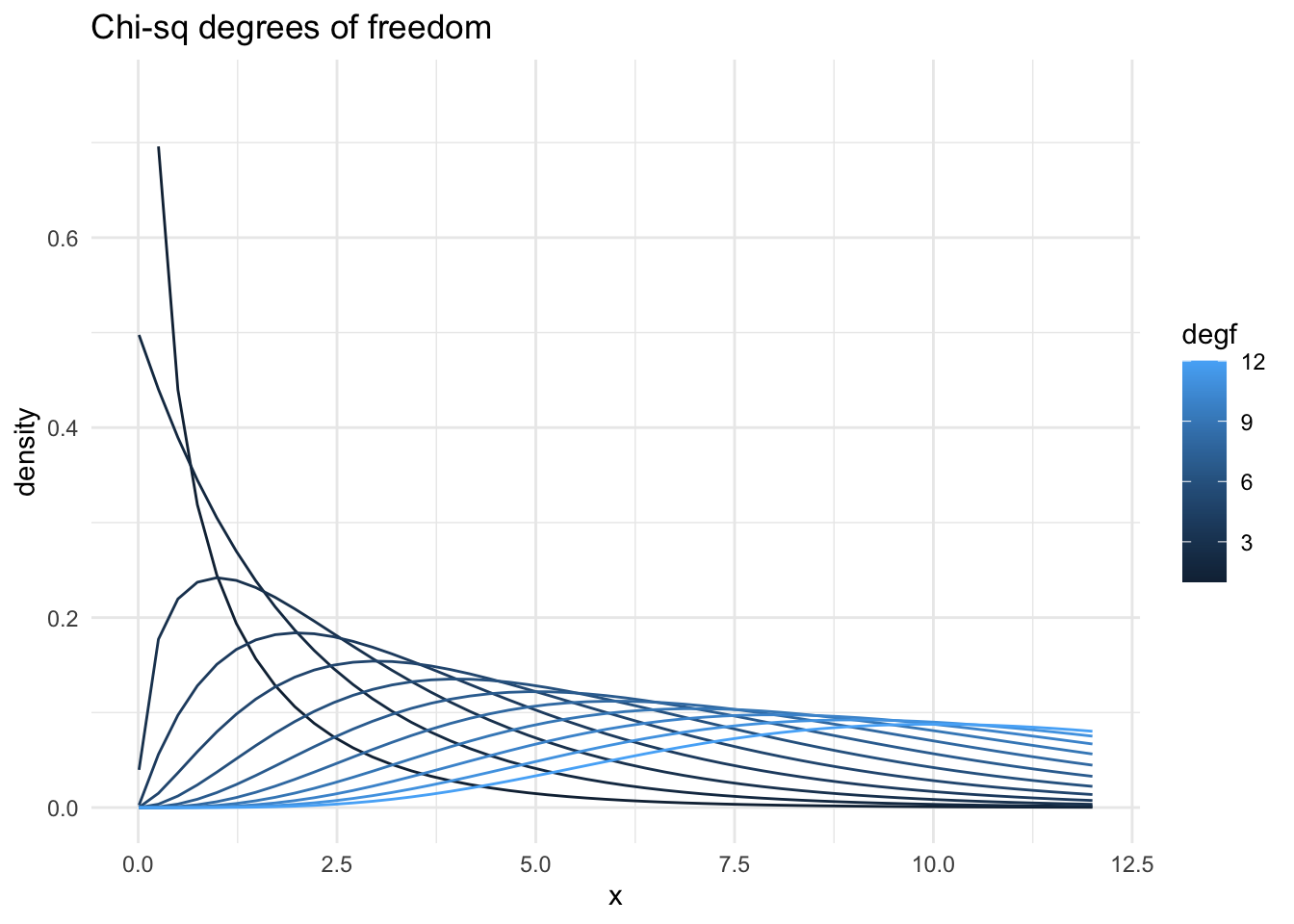
The origin of the \(\chi^2\) distribution is as the sum of independent squared standard normal variables, i.e. if

\(Y = Z_1^2 + Z_2^2 + \dots Z_n^2\), where \(Z_i \sim \mathcal{N}(0,1)\), then \(Y \sim \chi^2(n)\), a chi-squared distribution with \(n\) degrees of freedom. Note the relationship with the CLT: as more terms are added the chi-squared distribution (slowly) becomes more like the normal.

library(ggplot2)

dataf <- data.frame(x=rep(seq(from=0.01, to=12, length.out=50), times=12), degf=rep(1:12, each=50)) 
  
dataf$density <- apply(dataf, 1, function(x) dchisq(x[1],x[2]))

p <- ggplot(dataf,aes(x=x,y=density, group=degf, color=degf)) +
  geom_line() +
  ylim(0,0.75) + theme_minimal() +
  labs(title = "Chi-sq degrees of freedom")
p

If \(X \sim \mathcal{N}(\mu,\sigma^2)\), we can intuitively see how a chi-squared distribution is related to variance: \(S^2 = \frac{1}{n}\sum_{i=1}^{n}(X_i - \mu)^2\) which implies \(\frac{S^2}{\sigma^2}=\frac{1}{n}\sum_{i=1}^{n}(\frac{X_i - \mu}{\sigma})^2=\frac{1}{n}\sum_{i=1}^{n}Z_i^2\) where \(Z_i \sim \mathcal{N}(0,1)\). Note that in practice \(\mu\) is not known but estimated by the sample mean \(\bar{X}\) - hence the Bessel correction factor of \(\frac{1}{n-1}\) in the normal formula for sample variance and also, because there is one degree of freedom less (hand-wavy stats! but very typical that for each parameter we estimate we lose a degree of freedom), we have the result \[\frac{(n-1)S^2}{\sigma^2} \sim \chi^2(n-1)\] For a more formal proof see here

t Distribution

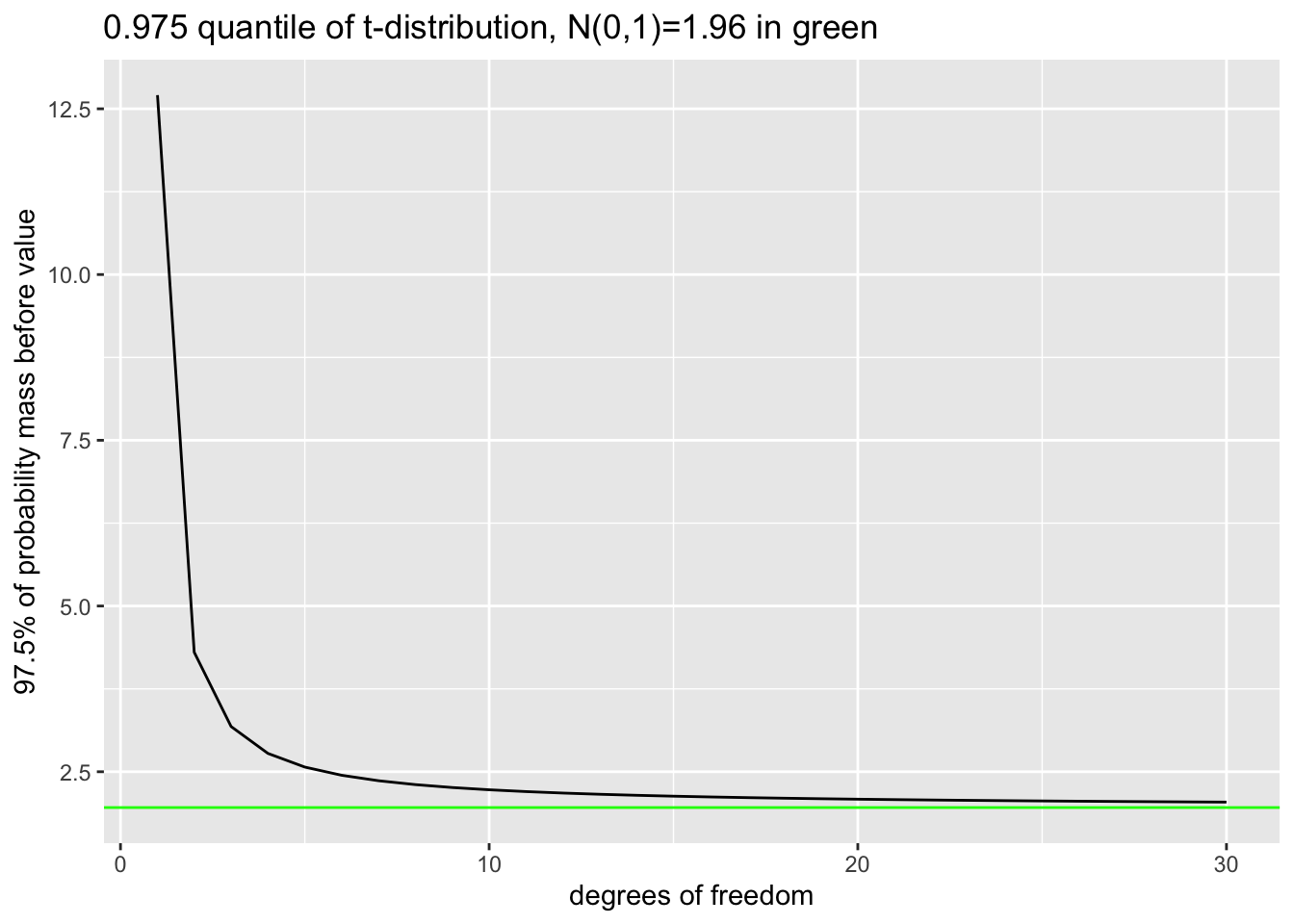
The \(t\) distribution is closely related to the normal distribution - it’s flatter, with more probability mass in the tails. As the degrees of freedom increase, it moves closer and closer to the standard normal, until \(t(\infty)=\mathcal{N}(0,1)\).

library(ggplot2)

tquant <- qt(0.975,1:30)
tdata <- data.frame(tquant,degfree=1:30)
q <- ggplot(tdata,aes(x=degfree, y=tquant)) +
  geom_line() +
  geom_hline(yintercept = qnorm(0.975),colour='green') +
  labs(title="0.975 quantile of t-distribution, N(0,1)=1.96 in green") +
  xlab("degrees of freedom") + ylab("97.5% of probability mass before value")
q

Having degrees of freedom is a clue that a \(\chi^2\) distribution might be involved somewhere, and indeed if \(Z \sim \mathcal{N}(0,1)\) and \(V \sim \chi^2(\nu)\) then \[ T = \frac{Z}{\sqrt{(V/\nu)}}\] has a \(t\)-distribution with \(\nu\) degrees of freedom.

Useful example: \(Z = (\bar{X_n}-\mu)(\sqrt\frac{n}{\sigma^2})\) is standard normal by the central limit theorem, and \(V = (n-1)\frac{S_n^2}{\sigma^2}\) is chi-squared with \((n-1)\) degrees of freedom as above, so: \[ T = \frac{Z}{\sqrt{V/(n-1)}} = (\bar{X_n}-\mu)\biggl(\sqrt\frac{n}{S_n^2}\biggr) \] has a \(t\)-distribution with (n-1) degrees of freedom, which is very useful because the unknown \(\sigma^2\) terms have cancelled out and \(S_n^2\) is the sample variance which we can calculate from the data.

F Distribution

The F distribution comes from the ratio of two chi-squared random variables. Recall from above that chi-squared is typically associated with estimating a variance parameter (like \(\sigma^2\)), and indeed we meet the F distribution when we wish to compare two variances. One classic example is checking the assumption of equal variance in a two sample \(t\)-test, or its more general version “ANOVA” - which is unsurprising if we know that ANOVA stands for analysis of variance.